Beautiful plots made via myTAI • myTAI

Gallery of different plots available with myTAI

Here are example outputs of plotting functions from myTAIv2.

We hope these plots can inspire your analysis!

Bulk RNA-seq data

example_phyex_set is an example BulkPhyloExpressionSet object.

To learn more about bringing your dataset into myTAI, follow this vignette here:
→ 📊

library(myTAI); library(S7); library(ggplot2); library(patchwork)
data("example_phyex_set")

myTAI plots can be modified as a ggplot2 object.

myTAI::plot_signature(example_phyex_set, 
                      show_p_val = TRUE, 
                      conservation_test = stat_flatline_test,
                      colour = "lavender") +
  # as the plots are ggplot2 objects, we can simply modify them using ggplot2
  ggplot2::labs(title = "Developmental stages of A. thaliana")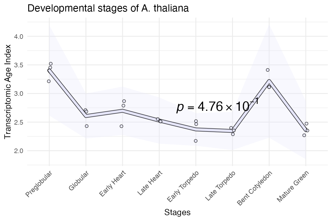

plot_signature function output with stat_flatline_test

module_info <- list(early = 1:3, mid = 4:6, late = 7:8)
myTAI::plot_signature(example_phyex_set,
                      show_p_val = TRUE,
                      conservation_test = stat_reductive_hourglass_test,
                      modules = module_info,
                      colour = "lavender")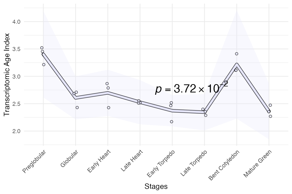

plot_signature function output with stat_reductive_hourglass_test

Transformation and robustness checks

See more here:
→ 🛡️

myTAI::plot_signature_transformed(
  example_phyex_set)

## Computing: [========================================] 100% (done)                         
## Computing: [========================================] 100% (done)                         
## Computing: [========================================] 100% (done)                         
## Computing: [========================================] 100% (done)                         
## Computing: [========================================] 100% (done)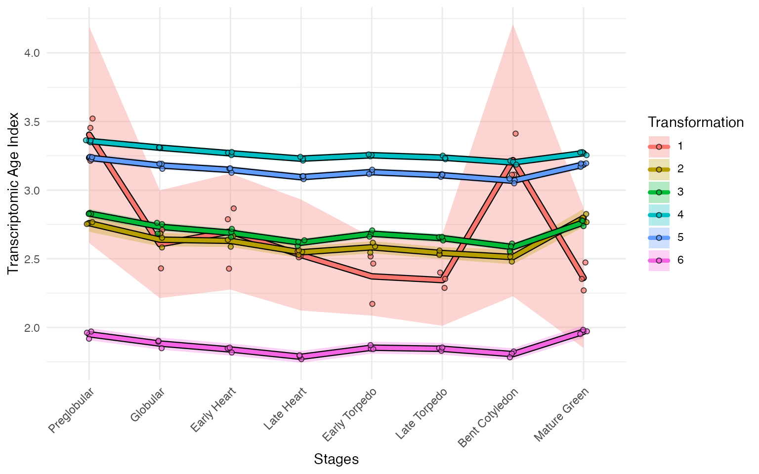

plot_signature_transformed function output

myTAI::plot_signature_gene_quantiles(
  example_phyex_set)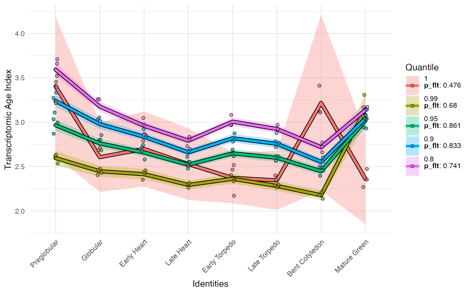

plot_signature_gene_quantiles function output

Statistical tests and plotting results

See more here:
→ 📈

myTAI::stat_flatline_test(
  example_phyex_set, plot_result = TRUE)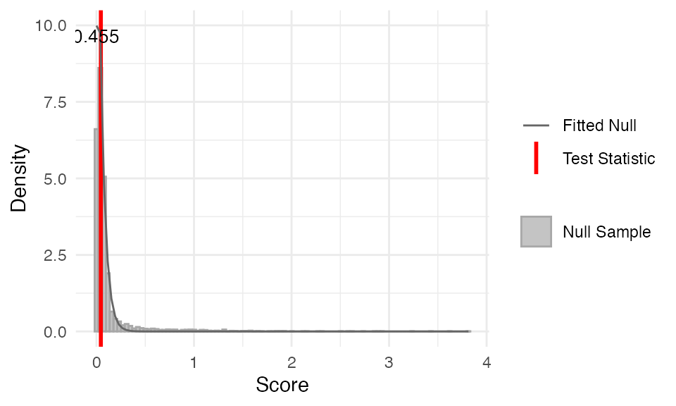

stat_flatline_test function output

## 
## Statistical Test Result
## =======================
## Method: Flat Line Test 
## Test statistic: 0.0446168 
## P-value: 0.4548801 
## Alternative hypothesis: greater 
## Data: Embryogenesis 2019

res_flt <- myTAI::stat_flatline_test(example_phyex_set, plot_result = FALSE)

myTAI::plot_cullen_frey(res_flt)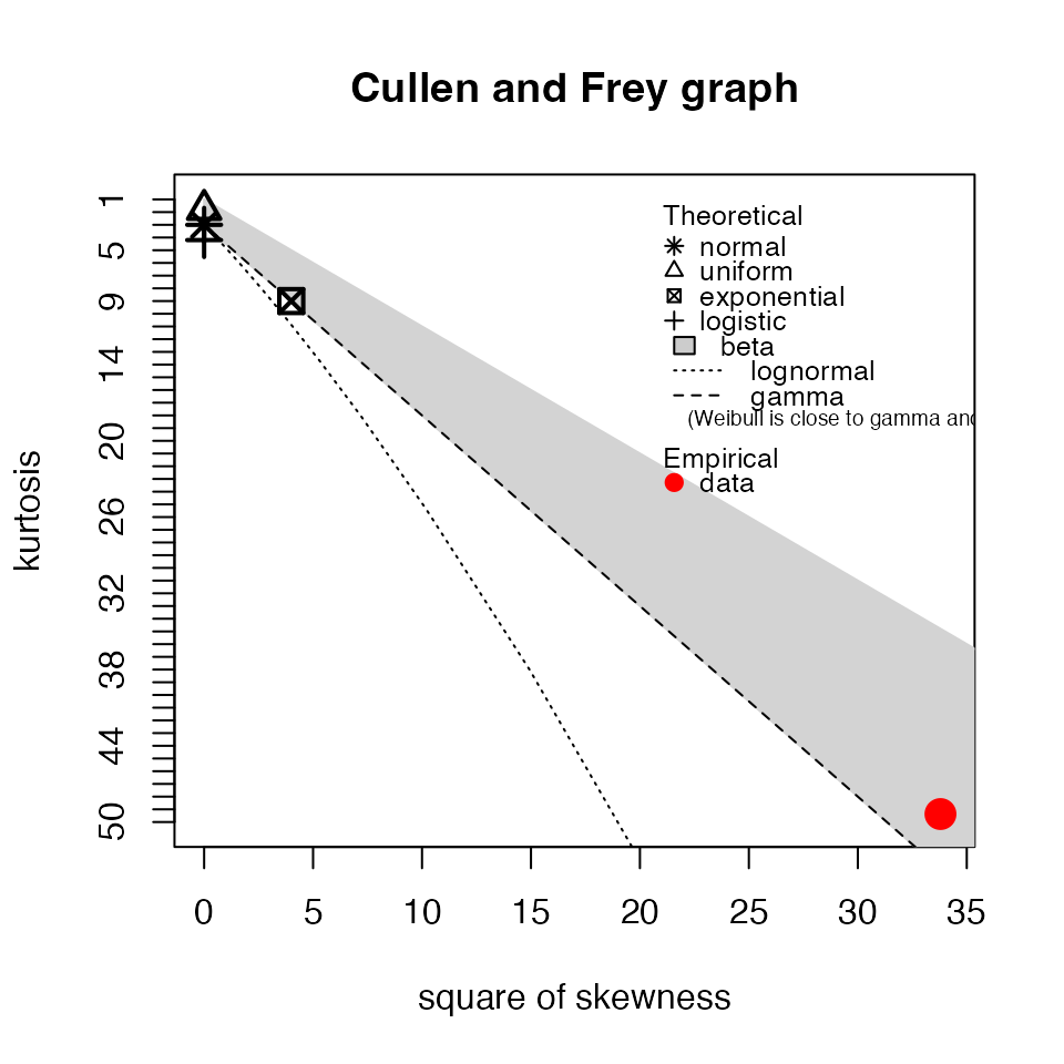

plot_cullen_frey function output for stat_flatline_test

## summary statistics
## ------
## min:  0.0001869433   max:  3.813752 
## median:  0.04687948 
## mean:  0.1172997 
## estimated sd:  0.2667466 
## estimated skewness:  5.813215 
## estimated kurtosis:  49.37137

myTAI::plot_null_txi_sample(res_flt) +
  ggplot2::guides(x =  guide_axis(angle = 90))

plot_null_txi_sample function output for stat_flatline_test

module_info <- list(early = 1:3, mid = 4:6, late = 7:8)
myTAI::stat_reductive_hourglass_test(
  example_phyex_set, plot_result = TRUE,
  modules = module_info)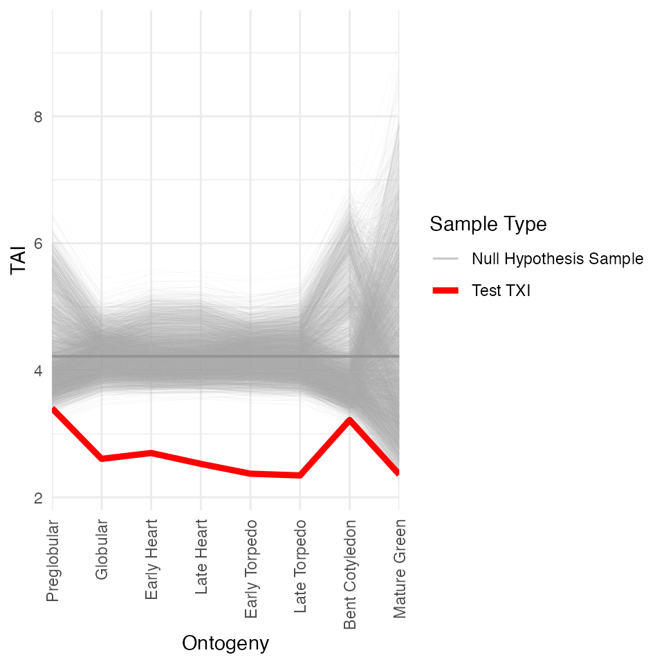

stat_reductive_hourglass_test function output

## 
## Statistical Test Result
## =======================
## Method: Reductive Hourglass Test 
## Test statistic: -0.03191036 
## P-value: 0.1962848 
## Alternative hypothesis: greater 
## Data: Embryogenesis 2019

Average gene expression level by phylostratum

myTAI::plot_strata_expression(example_phyex_set)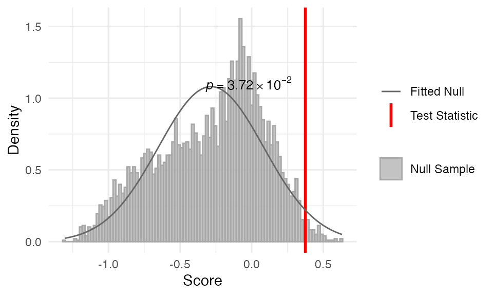

plot_strata_expression function output

plot_strata_expression with scaled y axis

myTAI::plot_strata_expression(example_phyex_set) +
  ggplot2::scale_y_log10() +
  ggplot2::labs(x = "Expression aggregated by mean (log-scaled)")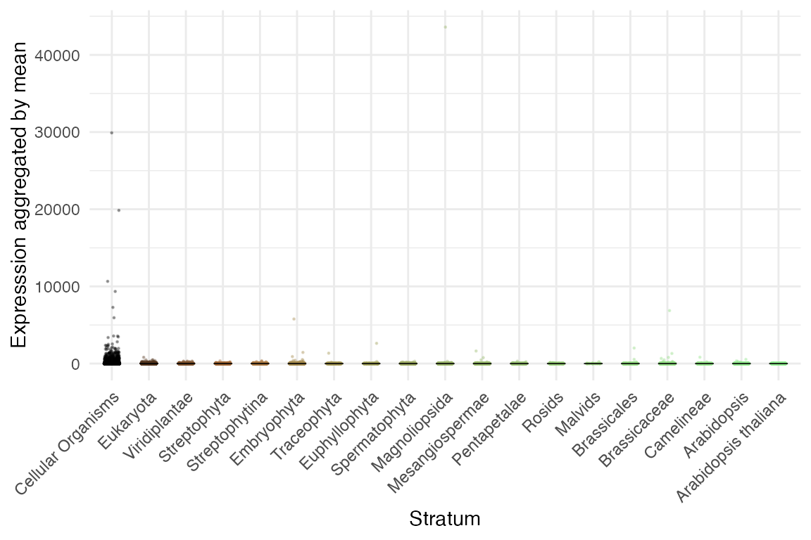

plot_strata_expression function output ggplot2

plot_strata_expression with explicit transformation

library(patchwork)
p1 <- myTAI::plot_strata_expression(example_phyex_set |> myTAI::tf(log1p))

# equivalent to 
p2 <- example_phyex_set |> myTAI::tf(log1p) |> myTAI::plot_strata_expression() 

p1+p2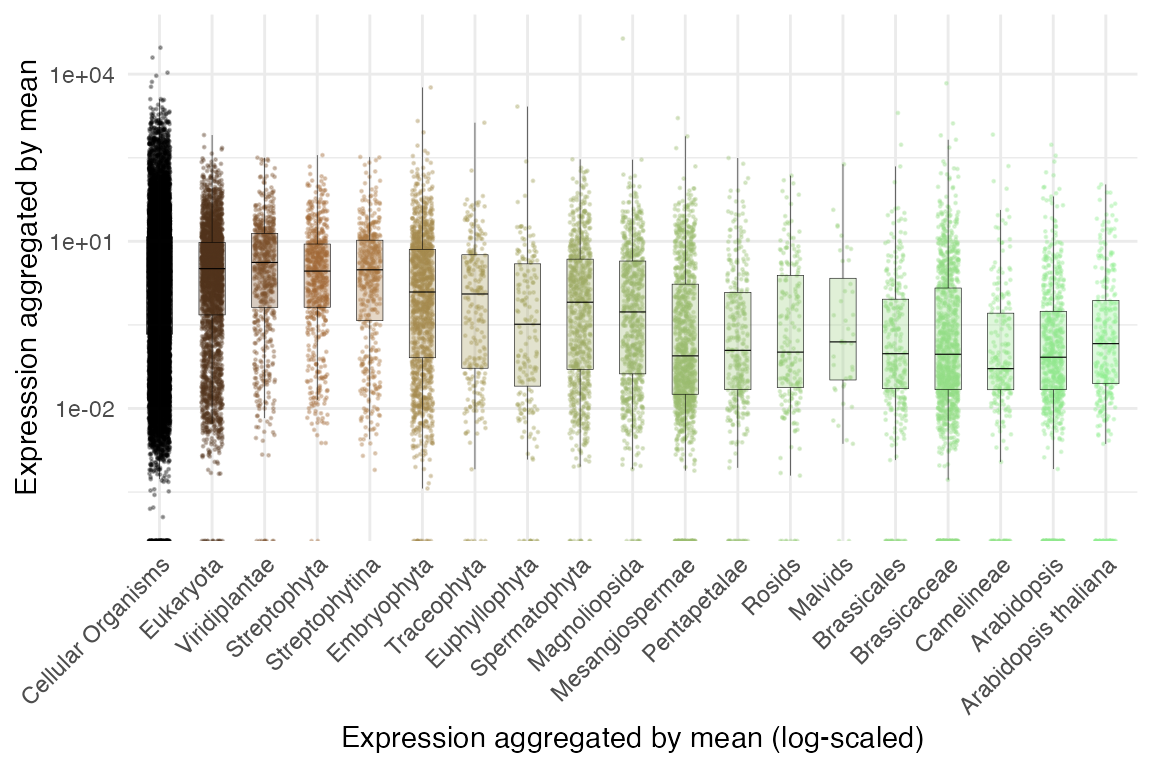

plot_strata_expression function output

As you can see, both plots are identical. This example demonstrates that there are multiple ways to achieve the same result through piping (|>) operator in R. |> is basically the same as %>%.

Contribution to the overall TAI by phylostratum

myTAI::plot_contribution(example_phyex_set)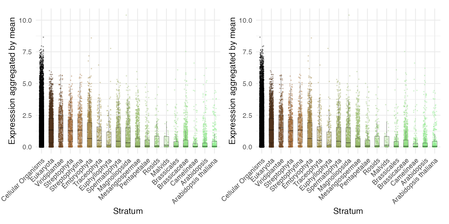

plot_contribution function output

Curious about methods to obtain gene age information? See more here:
→ 📚

For other analogous methods to assign evolutionary or expression information to each gene for TDI, TSI etc., see here:
→ 🧬

myTAI::plot_distribution_expression(example_phyex_set)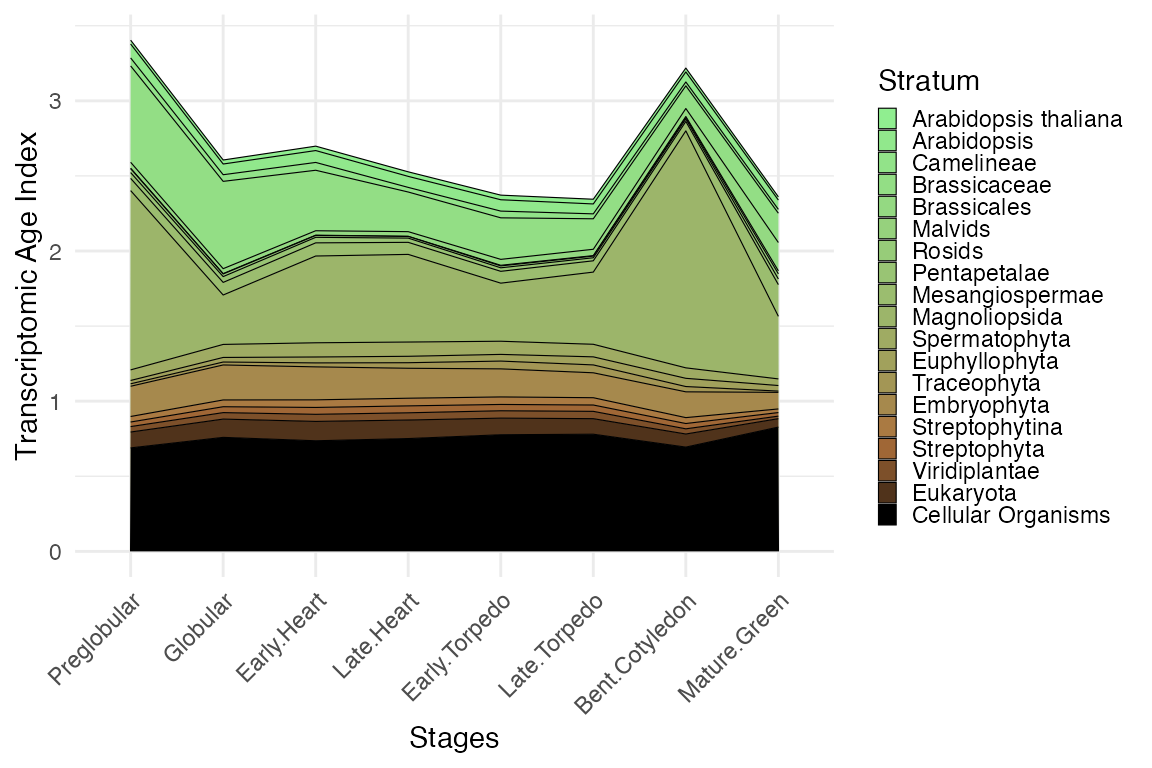

plot_distribution_expression function output

Contribution to the overall TAI by partial TAI (pTAI)

pTAI, or

$\mathrm{pTAI}_i = \frac{\mathrm{ps}_i \cdot e_{is}}{\sum_{i=1}^{n} e_{is}}$

where $e_{is}$ denotes the expression level of a given gene $) i$ in sample $s$ , ${ps}_i$ is its gene age assignment, and $n$ is the total number of genes, is the per-gene contribution to the overall TAI. (Summing pTAI across all genes gives in a given sample $s$ gives the overall ${TAI}_s$ )

pTAI QQ plot compares the partial TAI distributions of various developmental stages against a reference stage (default is stage 1).

myTAI::plot_distribution_pTAI_qqplot(example_phyex_set)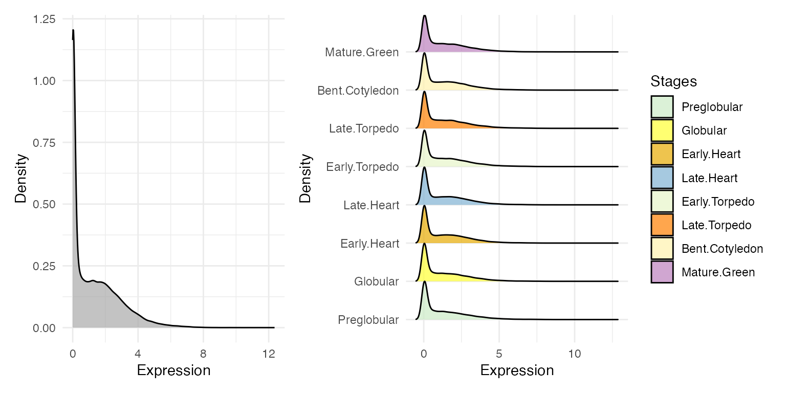

plot_distribution_pTAI_qqplot function output

Phylostratum distribution

myTAI::plot_distribution_strata(example_phyex_set@strata) /
myTAI::plot_distribution_strata(
  example_phyex_set@strata,
  selected_gene_ids = myTAI::genes_top_variance(example_phyex_set, p = 0.95),
  as_log_obs_exp = TRUE
) + plot_annotation(title = "Distribution of gene ages (top), Observed vs Expected plot of top 5% variance genes (bottom)")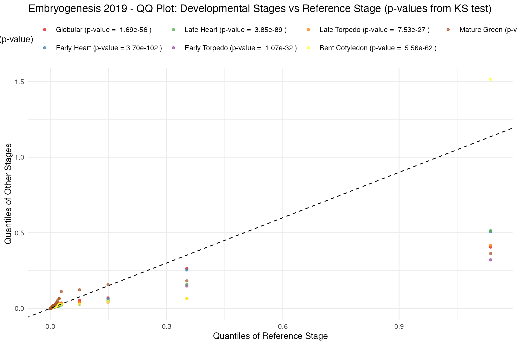

plot_distribution_strata function output

Expression heatmap

myTAI::plot_gene_heatmap(example_phyex_set)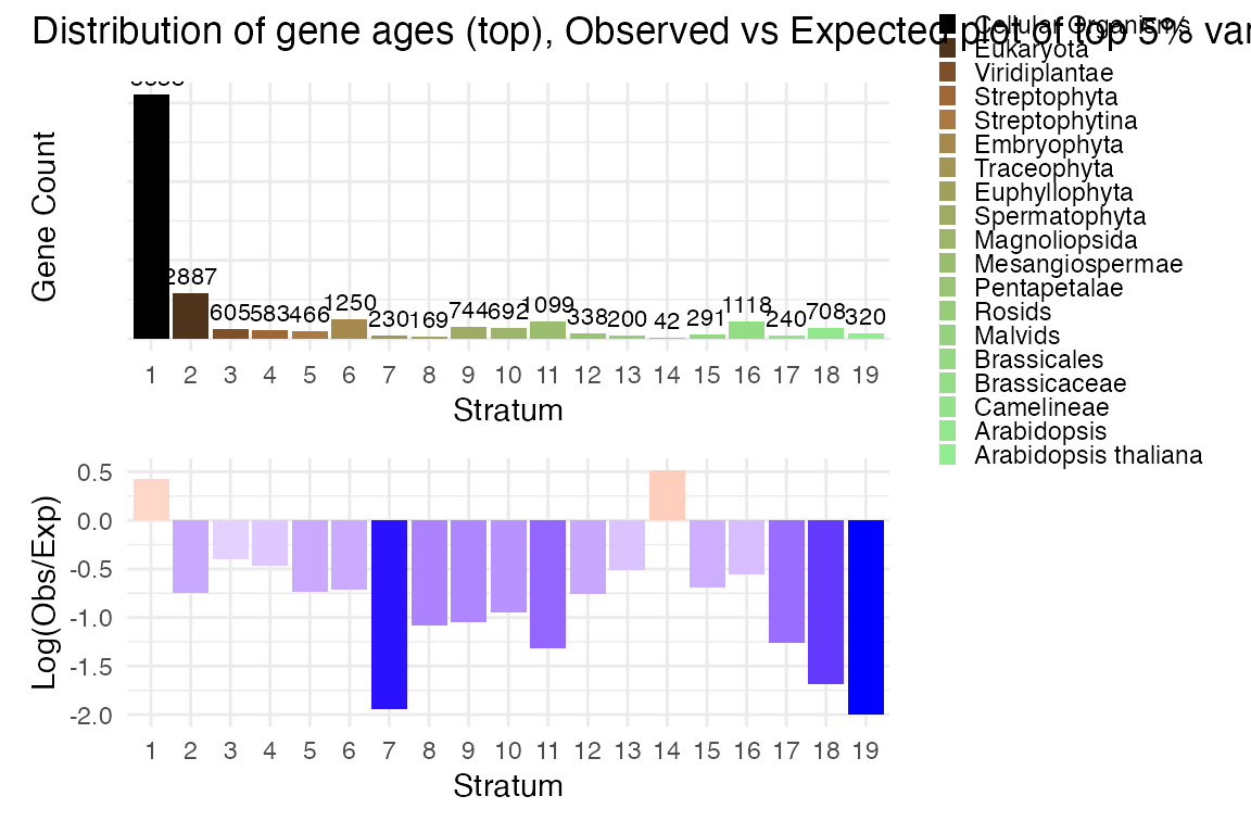

plot_gene_heatmap function output default

myTAI::plot_gene_heatmap(example_phyex_set, cluster_rows = TRUE, show_reps=TRUE, show_gene_ids=TRUE, top_p=0.005)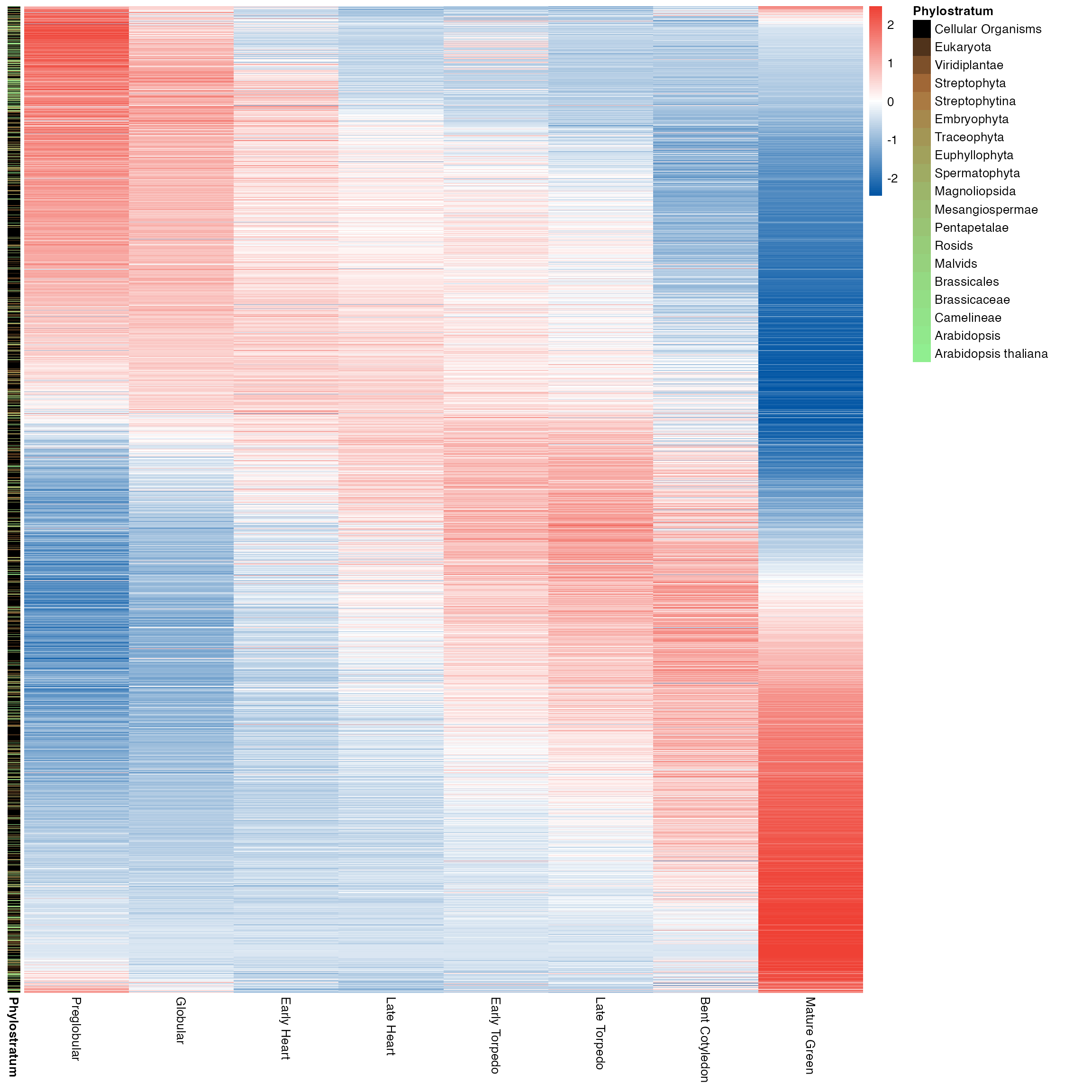

plot_gene_heatmap function output clustered

myTAI::plot_gene_heatmap(example_phyex_set, cluster_rows = TRUE, show_reps=TRUE, top_p=0.005, std=FALSE, show_gene_ids=TRUE)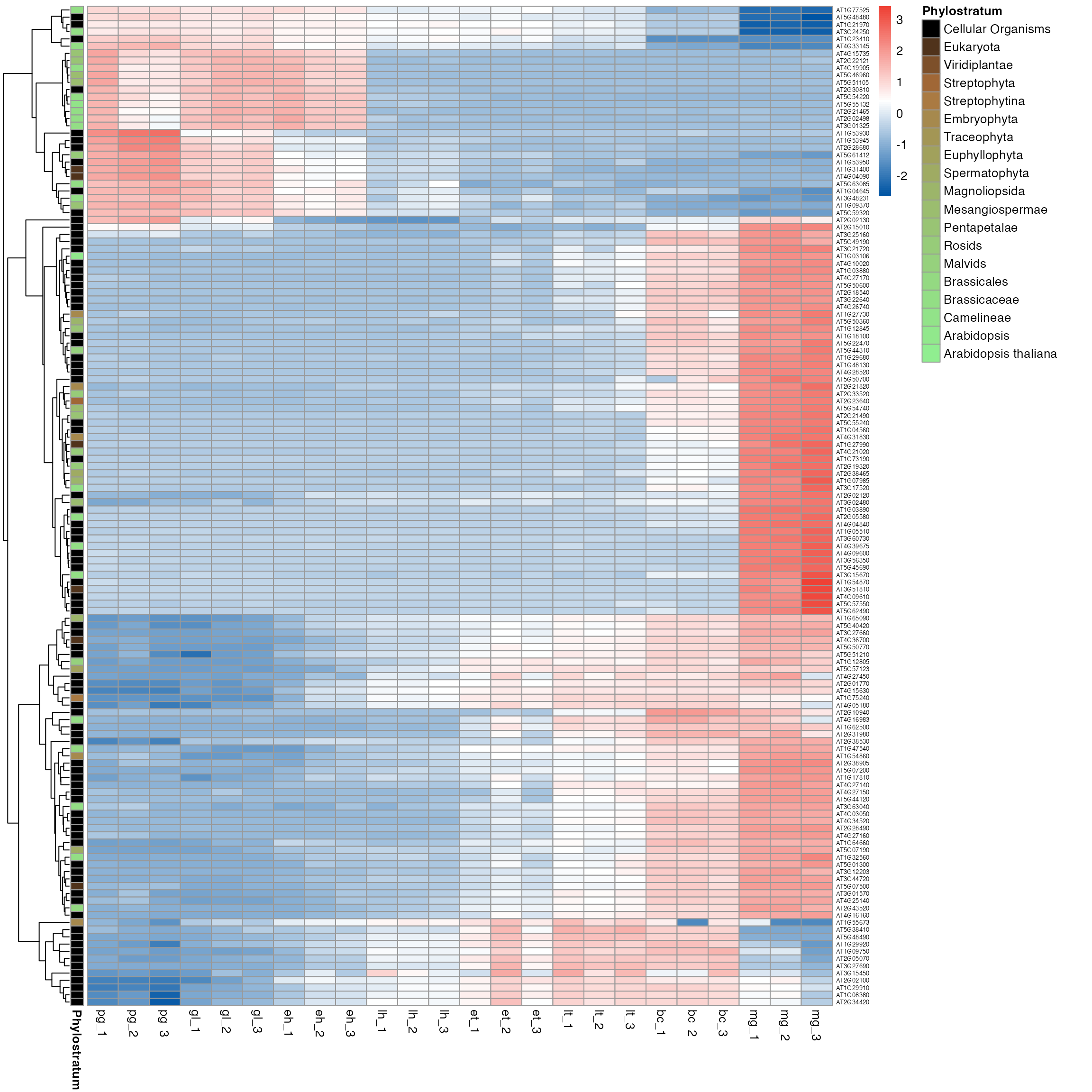

plot_gene_heatmap function output nonstd

Dimension reduction

At the gene level

myTAI::plot_gene_space(example_phyex_set)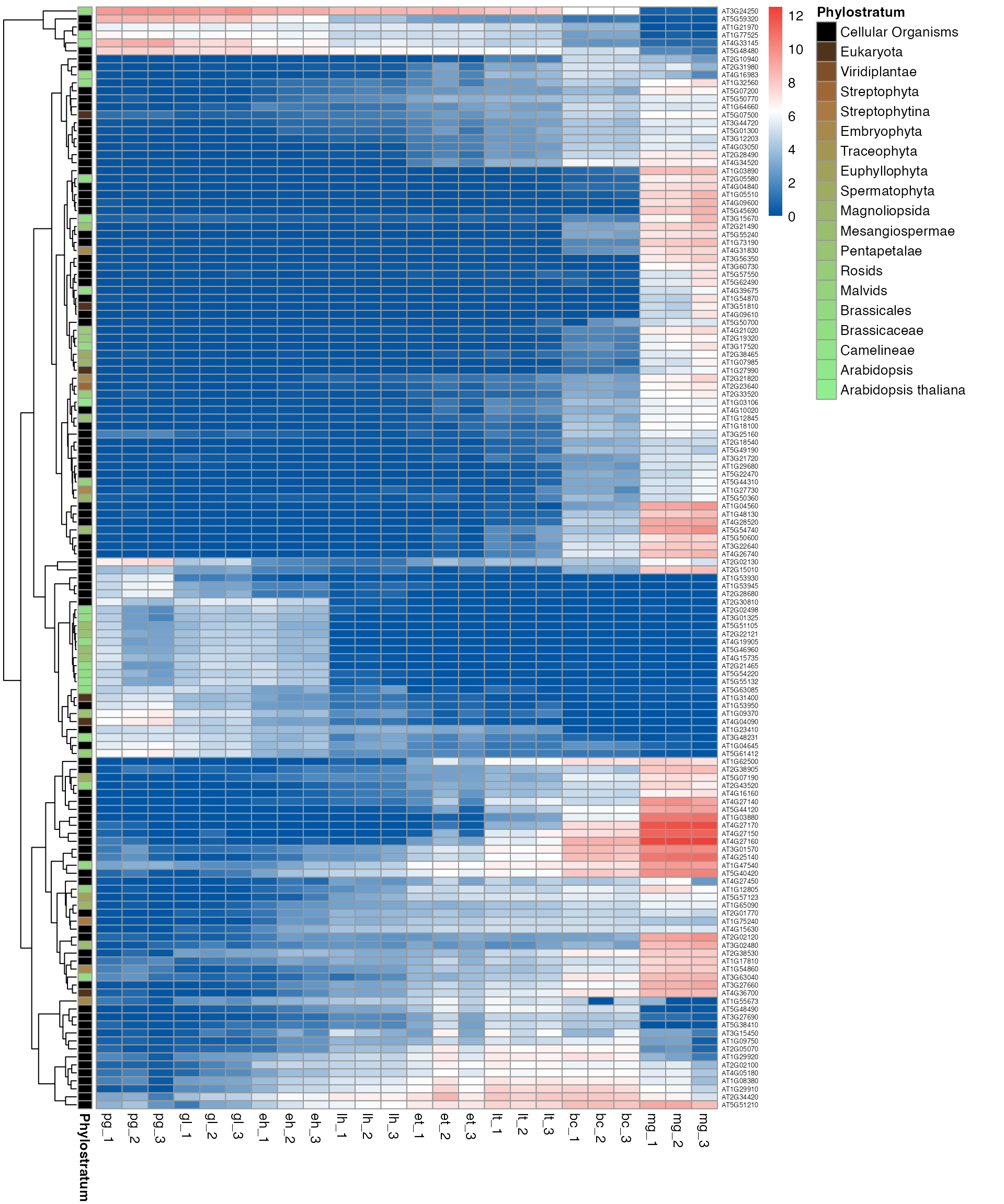

plot_gene_space function output

myTAI::plot_gene_space(example_phyex_set,colour_by = "strata")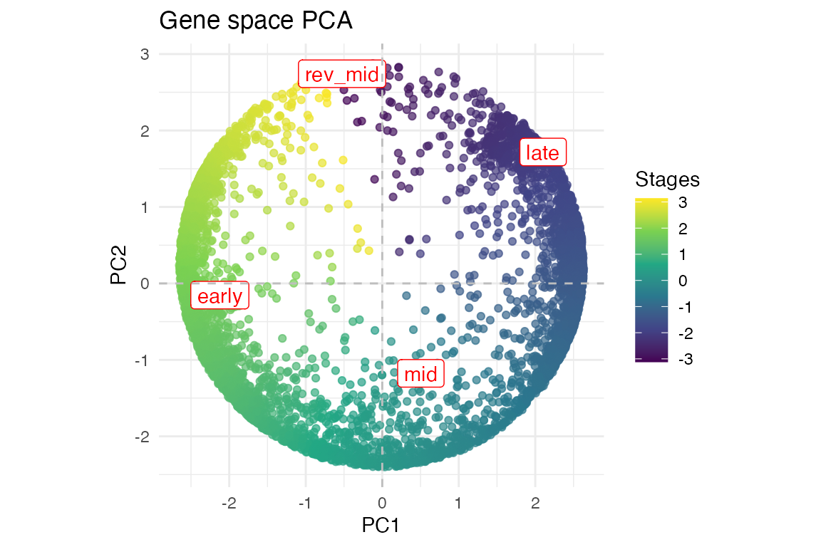

plot_gene_space function output by strata

At the sample level

myTAI::plot_sample_space(example_phyex_set) | myTAI::plot_sample_space(example_phyex_set, colour_by = "TXI")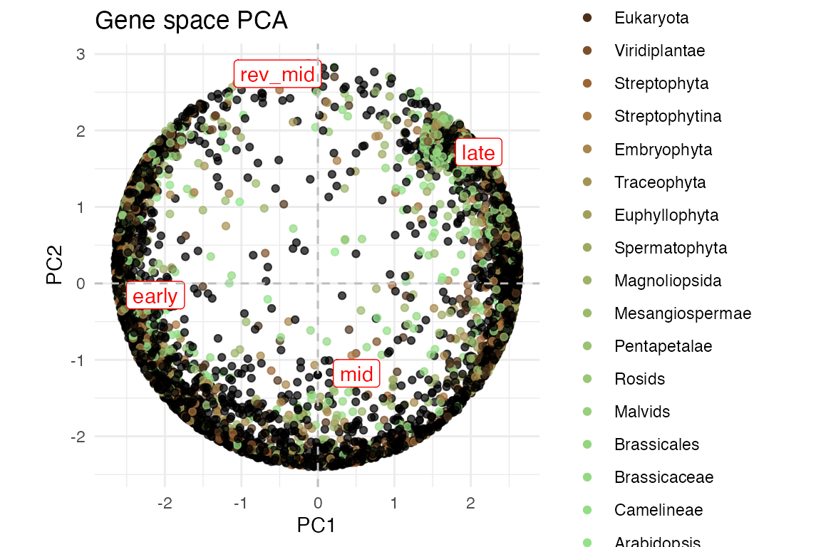

plot_sample_space function output by TXI

# we can even do a UMAP
myTAI::plot_sample_space(example_phyex_set, method = "UMAP")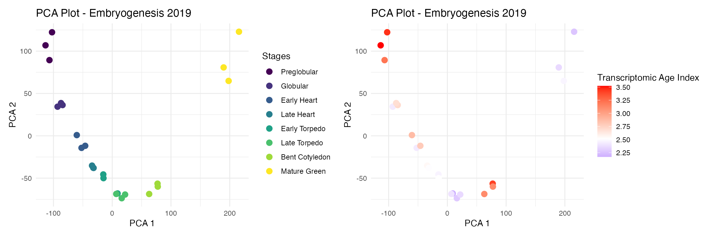

plot_sample_space function output by TXI

Inspecting mean-variance relationship

# highlighting top variance genes
top_var_genes <- myTAI::genes_top_variance(example_phyex_set, p = 0.9995)
p1 <- myTAI::plot_mean_var(example_phyex_set)
p2 <- myTAI::plot_mean_var(example_phyex_set, 
                     highlight_genes = top_var_genes)

p1 + p2 + plot_annotation(title = "Mean-variance: simple vs. highlighted top variance genes")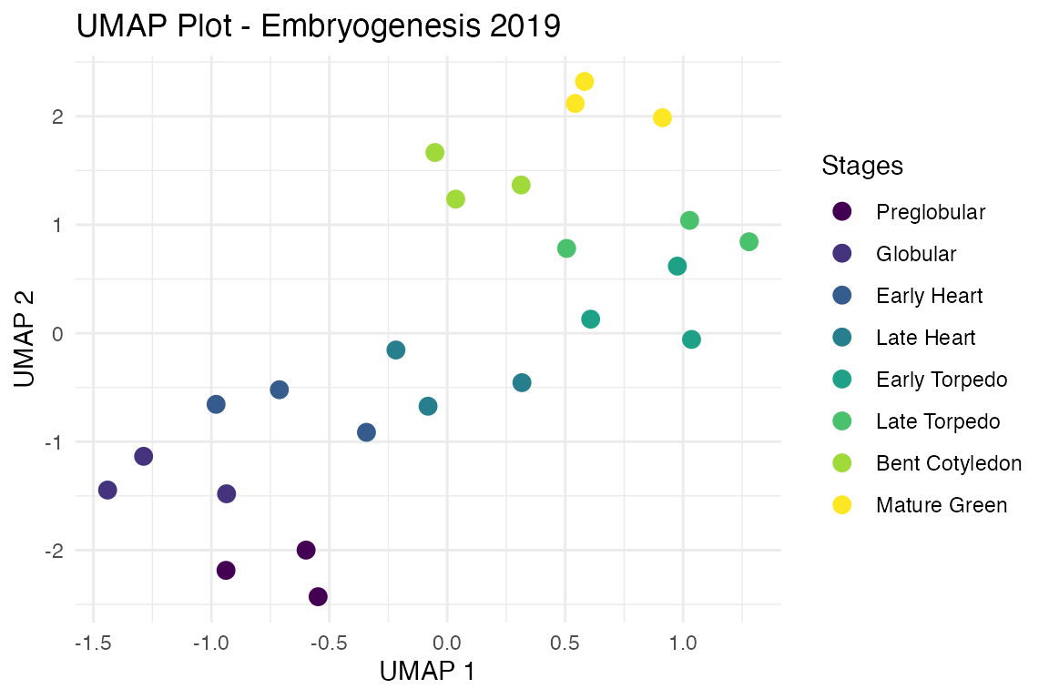

plot_mean_var function output simple vs highlighted

# with log transform and colouring by phylostratum
myTAI::plot_mean_var(example_phyex_set |> myTAI::tf(log1p), 
                     colour_by = "strata") +
  ggplot2::guides(colour = guide_legend(ncol=2))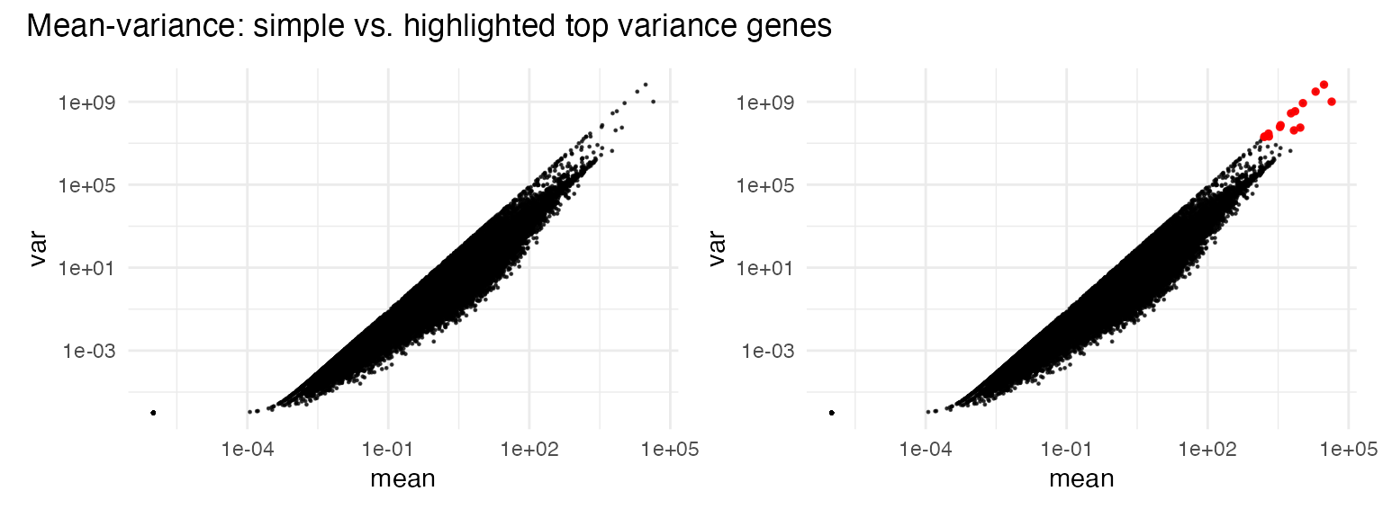

plot_gene_space function output log transform coloured by strata

Individual gene expression profiles

# side by side: manual coloring vs strata coloring
p1 <- myTAI::plot_gene_profiles(example_phyex_set, max_genes = 10, colour_by = "manual")
p2 <- myTAI::plot_gene_profiles(example_phyex_set, max_genes = 10, colour_by = "strata")

p1 + p2 + plot_annotation(title = "Gene profiles: manual vs. strata coloring")

plot_gene_profiles function output manual vs strata coloring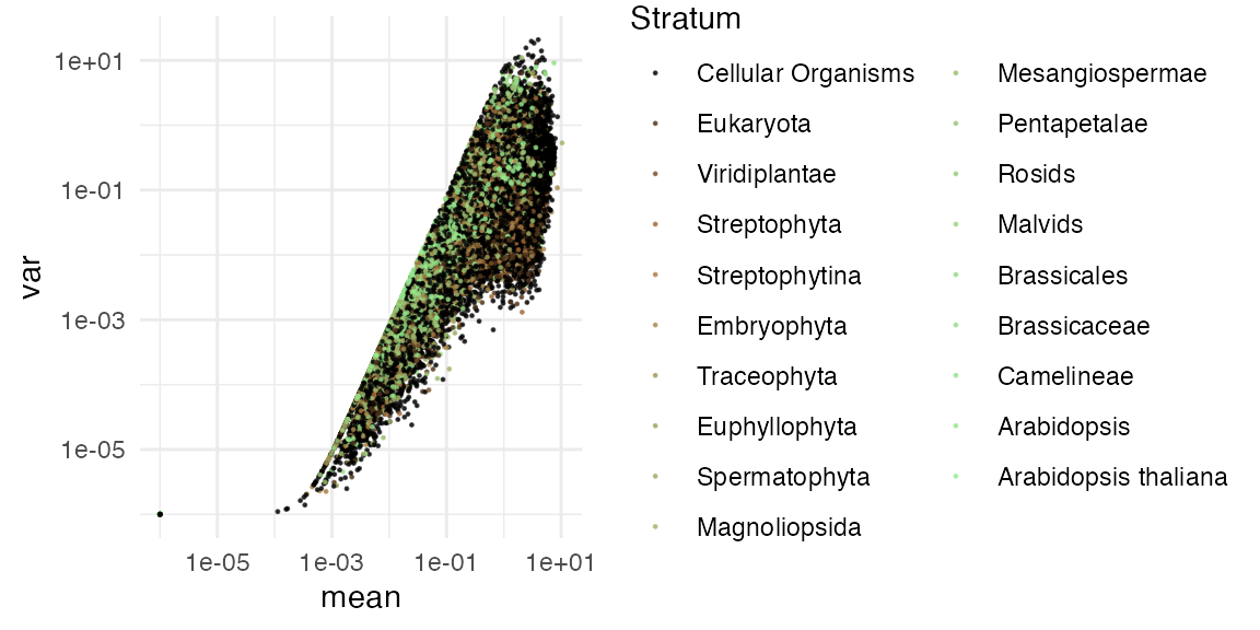

# stage colouring with standardized log transformation
myTAI::plot_gene_profiles(example_phyex_set, max_genes = 10, 
                          transformation = "std_log", colour_by = "stage")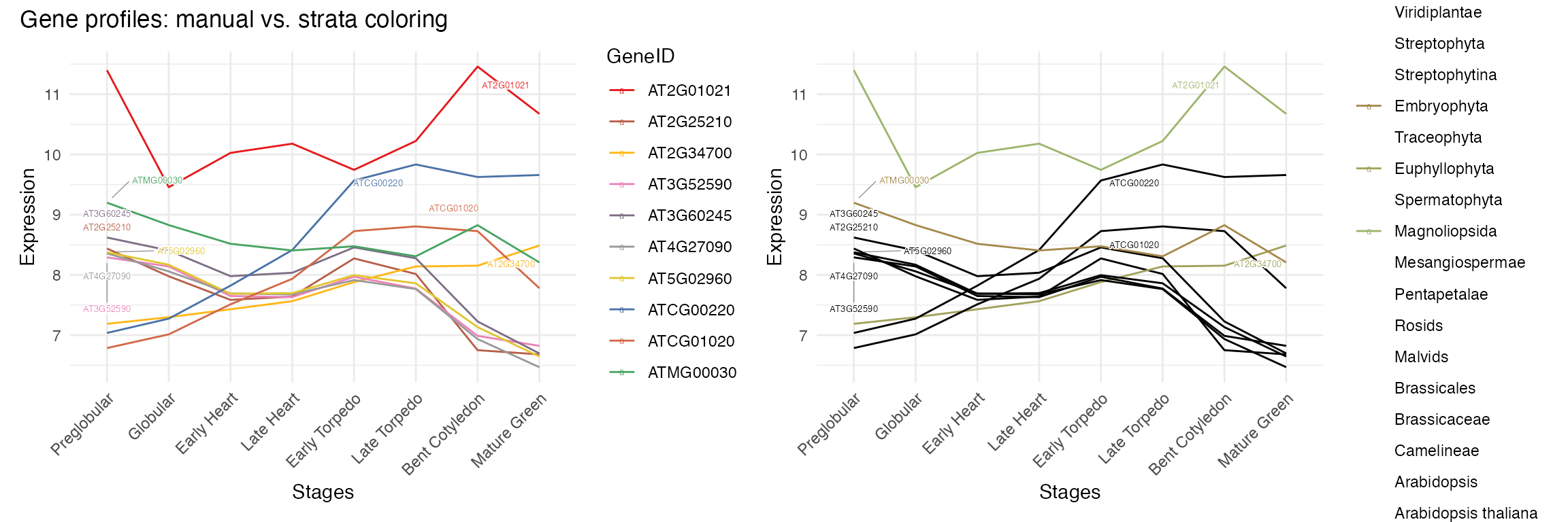

plot_gene_profiles function output stage std_log transformation

# faceted by phylostratum
myTAI::plot_gene_profiles(example_phyex_set, max_genes = 1000, 
                          colour_by = "strata", facet_by_strata = TRUE, show_set_mean = TRUE,
                          show_labels = FALSE)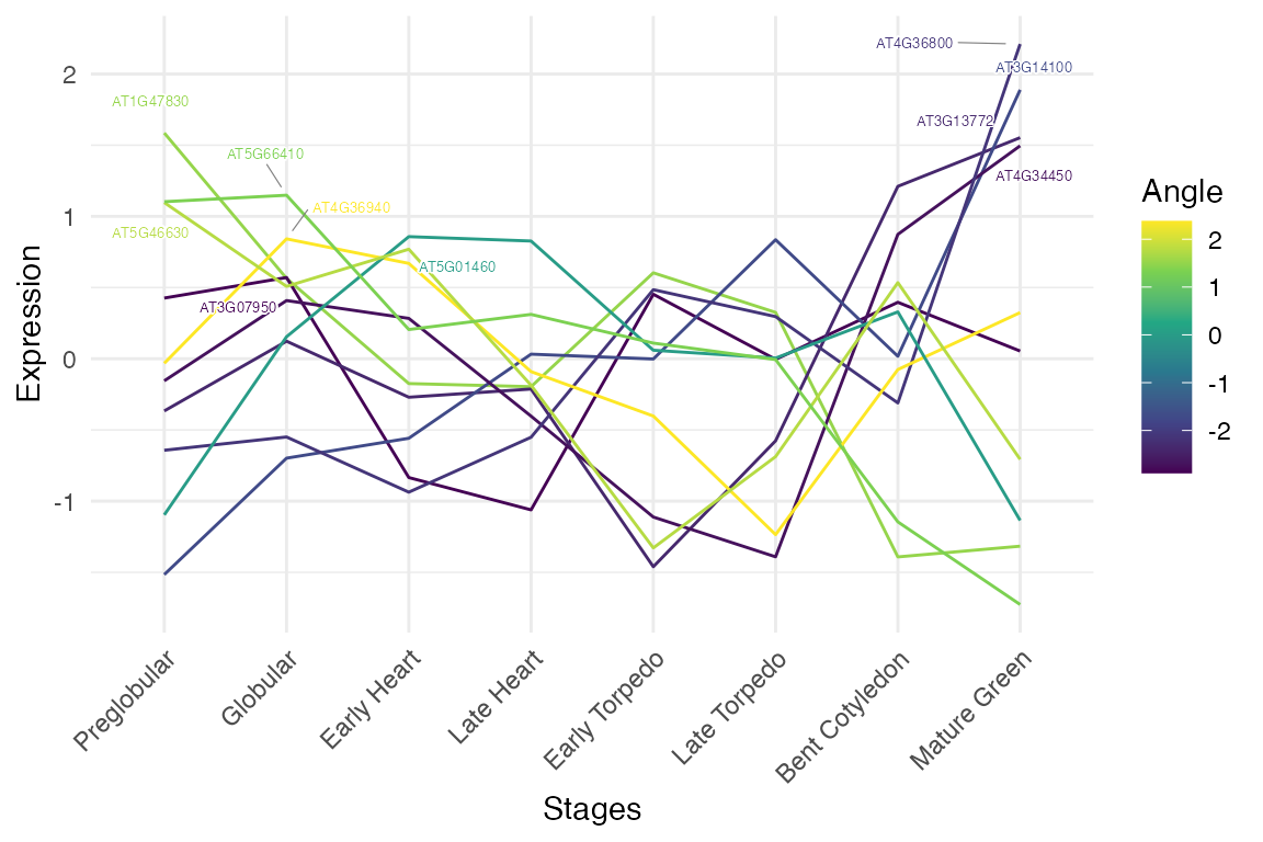

plot_gene_profiles function output faceted by strata

These plots are examples of plots that myTAIv2 can generate. To check out the functions, use ? before the function (i.e. ?myTAI::plot_mean_var().

You can also find a list of plotting functions in Reference.

Single cell RNA-seq data

Most of the plotting functions shown above also apply for single cell RNA-seq data, as long as it is a ScPhyloExpressionSet object.

Let’s create an example single-cell dataset and explore the plotting capabilities:

# Load example single-cell data
data(example_phyex_set_sc)

example_phyex_set_sc

## PhyloExpressionSet object
## Class: myTAI::ScPhyloExpressionSet 
## Name: Single Cell Example 
## Species: Example Species 
## Index type: TXI 
## Cell Type : TypeA, TypeB, TypeC 
## Number of genes: 100 
## Number of cell type : 3 
## Number of phylostrata: 10 
## Total cells: 1000 
## Cells per type:
## 
## TypeA TypeB TypeC 
##   341   335   324 
## Available metadata:
##   groups: TypeA, TypeB, TypeC
##   day: Day1, Day3, Day5, Day7
##   condition: Control, Treatment
##   batch: Batch1, Batch2, Batch3

# Check available identities
cat("Available identities for plotting:\n")

## Available identities for plotting:

print(example_phyex_set_sc@available_idents)

## [1] "groups"    "day"       "condition" "batch"

# Set up custom color schemes for better visualization
day_colors <- c("Day1" = "#3498db", "Day3" = "#2980b9", "Day5" = "#1f4e79", "Day7" = "#0d2a42")
condition_colors <- c("Control" = "#27ae60", "Treatment" = "#e74c3c")
group_colors <- c("TypeA" = "#e74c3c", "TypeB" = "#f39c12", "TypeC" = "#9b59b6")

example_phyex_set_sc@idents_colours[["day"]] <- day_colors
example_phyex_set_sc@idents_colours[["condition"]] <- condition_colors
example_phyex_set_sc@idents_colours[["groups"]] <- group_colors

Single-cell signature plots

# Basic signature plot showing TXI distribution across cell types
myTAI::plot_signature(example_phyex_set_sc)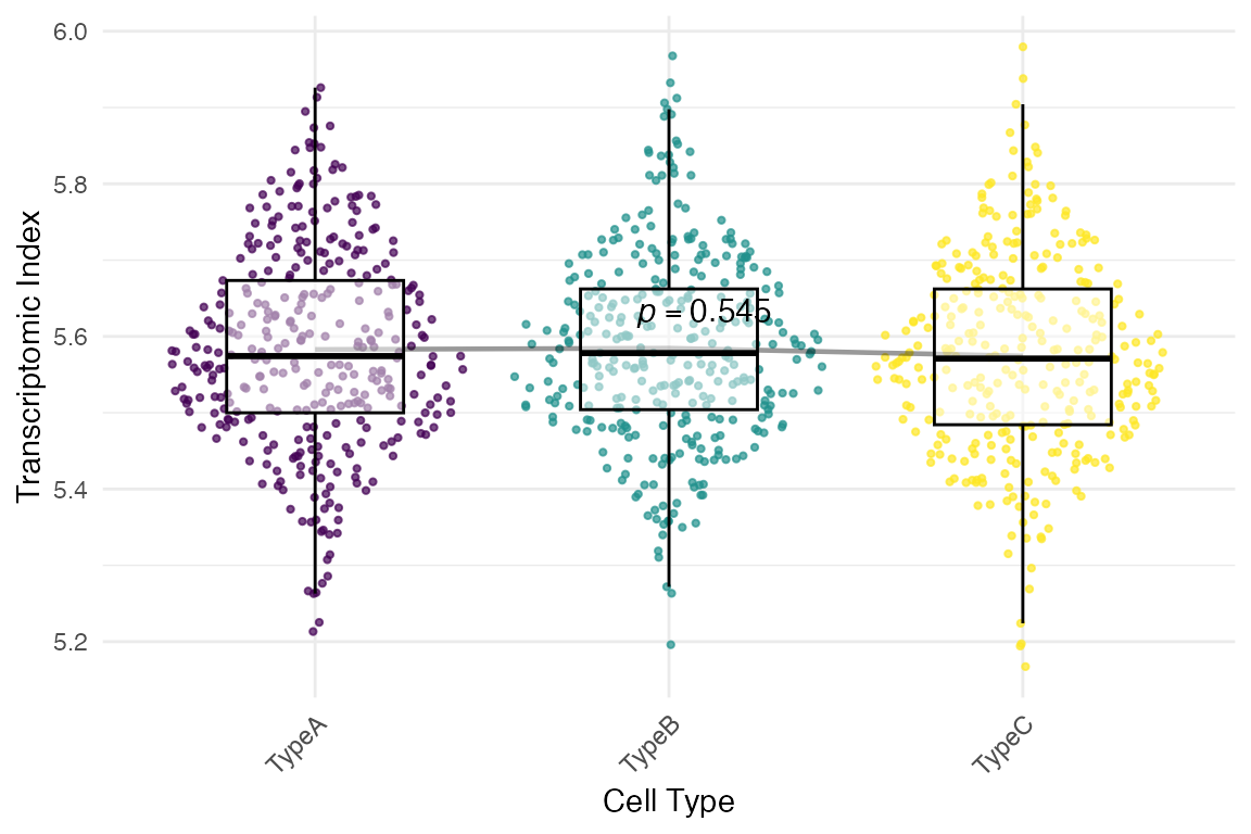

plot_signature single-cell basic

# Plot without showing individual cells (just means)
myTAI::plot_signature(example_phyex_set_sc, show_reps = FALSE)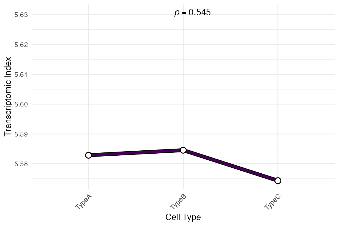

plot_signature single-cell without individual cells

# Plot TXI distribution by developmental day instead of cell type
myTAI::plot_signature(example_phyex_set_sc, primary_identity = "day", show_p_val = FALSE)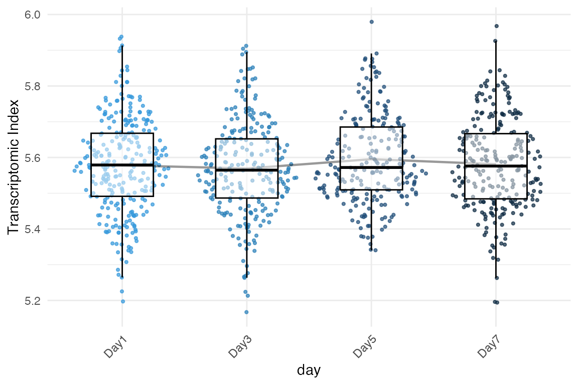

plot_signature single-cell by day

# Plot TXI distribution by experimental condition
myTAI::plot_signature(example_phyex_set_sc, primary_identity = "condition", show_p_val=FALSE)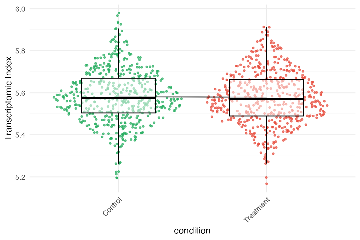

plot_signature single-cell by condition

You can use a secondary identity for either coloring or faceting to create more informative plots:

# Plot by day, colored by condition
myTAI::plot_signature(example_phyex_set_sc, 
                     primary_identity = "day", 
                     secondary_identity = "condition",
                     show_p_val=FALSE)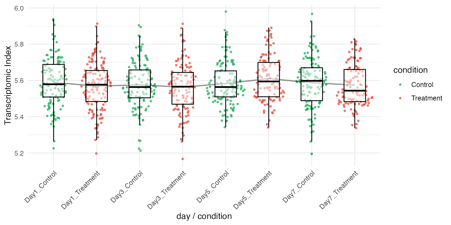

plot_signature single-cell with secondary coloring

# Plot by day, faceted by condition
myTAI::plot_signature(example_phyex_set_sc, 
                     primary_identity = "day", 
                     secondary_identity = "batch",
                     facet_by_secondary = TRUE,
                     show_p_val = FALSE)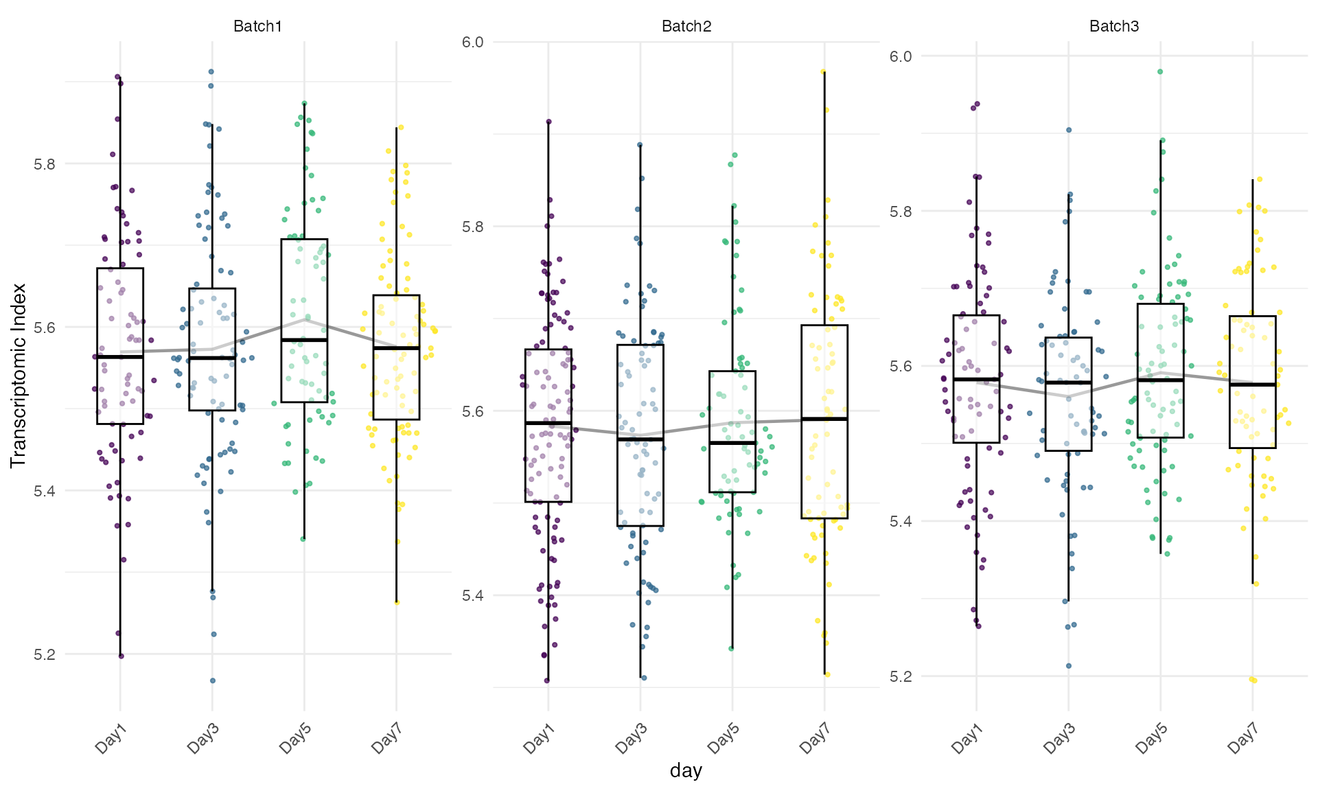

plot_signature single-cell with faceting

Other single-cell visualizations

The gene heatmap function also works with single-cell data and can show individual cells or be aggregated:

# Gene heatmap for single-cell data (aggregated by cell type)
myTAI::plot_gene_heatmap(example_phyex_set_sc, top_p = 0.1, cluster_rows=TRUE)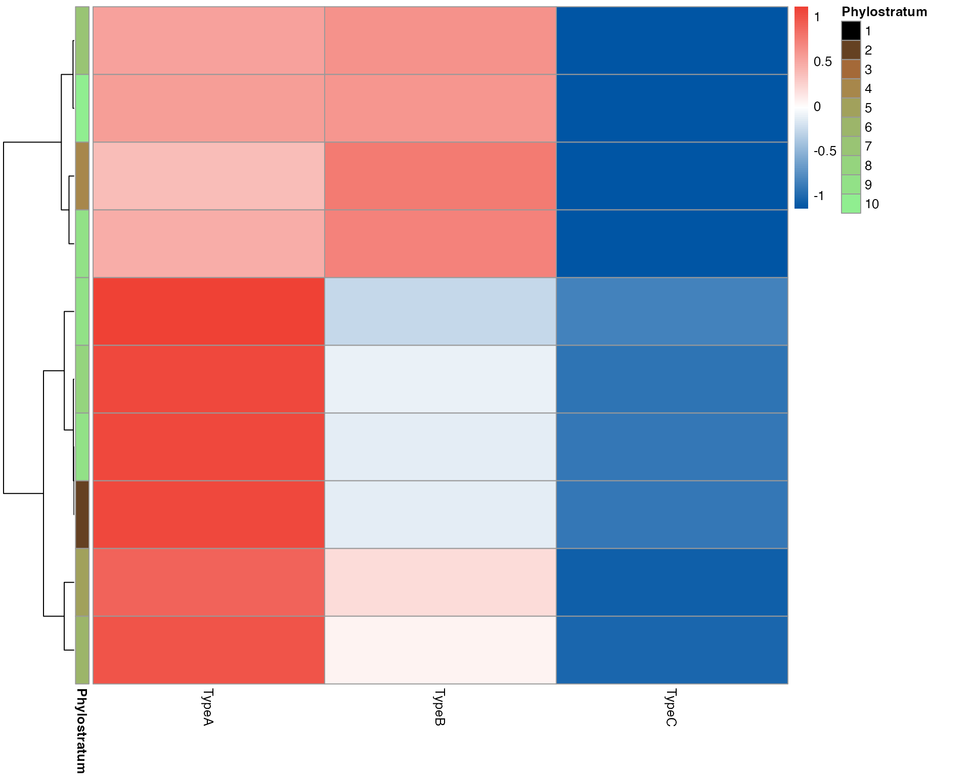

plot_gene_heatmap single-cell

# Gene heatmap showing individual cells (subsampled)
myTAI::plot_gene_heatmap(example_phyex_set_sc, show_reps = TRUE, max_cells_per_type = 10, top_p = 0.05, cluster_rows=TRUE)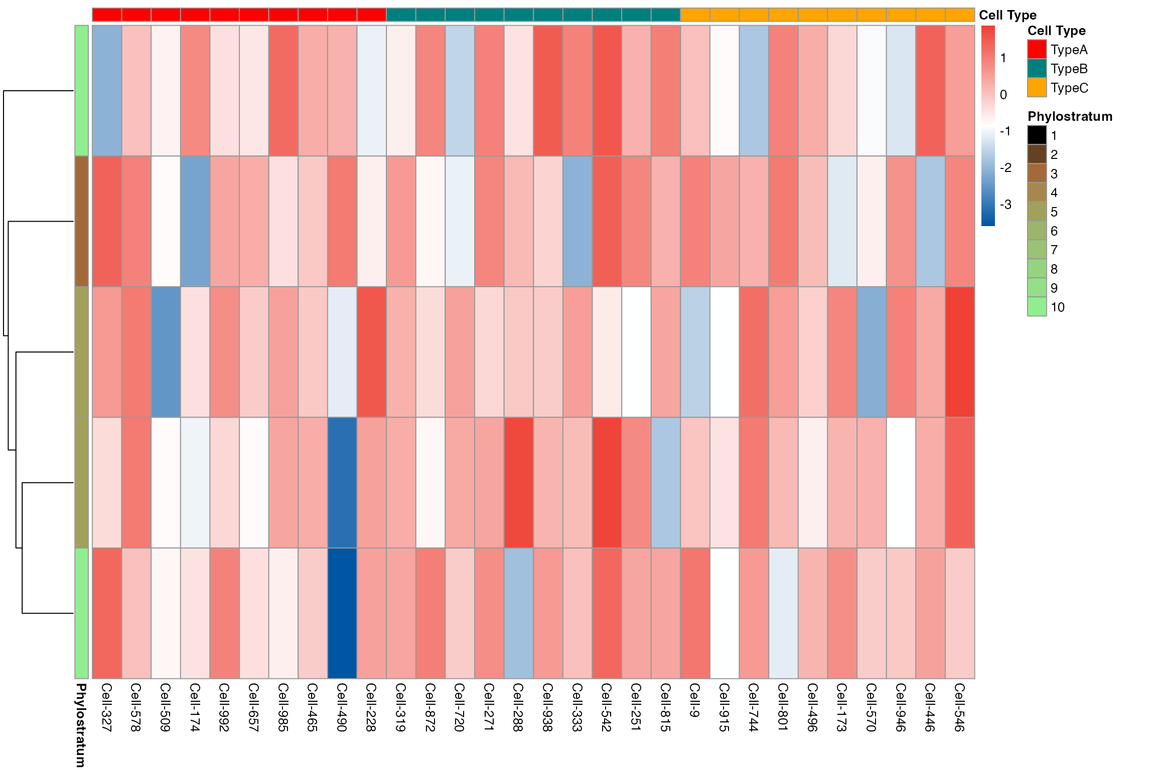

plot_gene_heatmap single-cell with individual cells

# Change identity to "day" and plot heatmap grouped by developmental time
example_sc_by_day <- example_phyex_set_sc
example_sc_by_day@selected_idents <- "day"
myTAI::plot_gene_heatmap(example_sc_by_day, show_reps = TRUE, max_cells_per_type = 8, top_p = 0.05, cluster_rows=TRUE, show_gene_ids=TRUE, std=FALSE)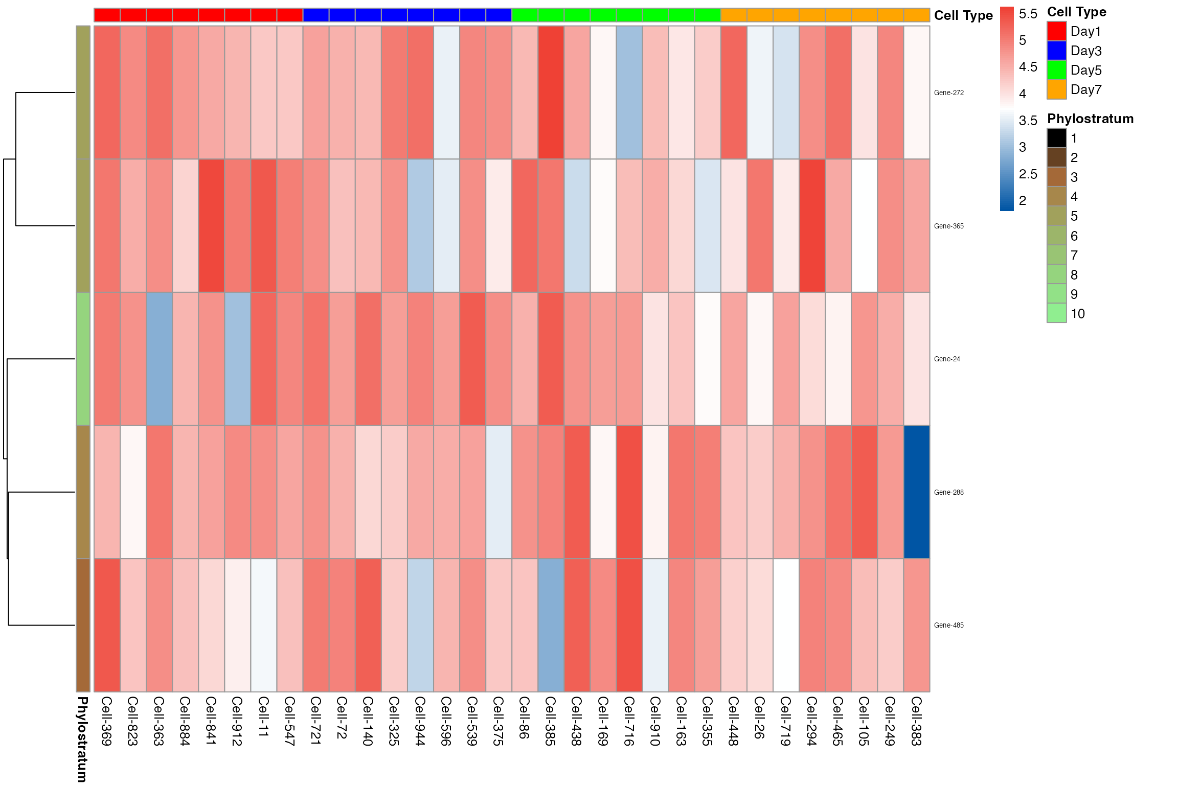

plot_gene_heatmap single-cell grouped by day

Single-cell plotting tips:

Use primary_identity to specify which metadata column to plot on the x-axis
Use secondary_identity with facet_by_secondary = TRUE for faceted plots
Use secondary_identity without faceting for colour-coded plots
Set custom colors with set_identity_colours()
Check available metadata columns with available_identities()

Plot away!