Bring your datasets into myTAI
Source:vignettes/phylo-expression-object.Rmd
phylo-expression-object.RmdS7 BulkPhyloExpressionSet and ScPhyloExpressionSet objects
Starting from myTAIv2, we moved on from the traditional
data.frame to the new S7 OOP system
to facilitate fast and flexible computation for evolutionary
transcriptomics analyses.
To illustrate this, we will use the example data
example_phyex_set. The BulkPhyloExpressionSet
and ScPhyloExpressionSet objects are designed to store gene
expression data along with associated metadata such as gene age
information (or phylorank), experiment
type and other relevant properties.
We will first focus on the BulkPhyloExpressionSet
object, which is for bulk RNA-seq data.
# inspect the object
example_phyex_set
More on S7 and the BulkPhyloExpressionSet
object
S7::prop_names(example_phyex_set)Show output
##  [1] "strata"                        "strata_values"
##  [3] "expression"                    "groups"
##  [5] "name"                          "species"
##  [7] "index_type"                    "identities_label"
##  [9] "expression_collapsed"          "gene_ids"
## [11] "identities"                    "sample_names"
## [13] "num_identities"                "num_samples"
## [15] "num_genes"                     "num_strata"
## [17] "index_full_name"               "group_map"
## [19] "TXI"                           "TXI_sample"
## [21] "null_conservation_sample_size" ".null_conservation_txis"
## [23] "null_conservation_txis"        ".bootstrapped_txis"
## [25] "bootstrapped_txis"
# let's explore the properties using @
# for example:
example_phyex_set@strata |> head()
example_phyex_set@gene_ids |> head()
example_phyex_set@expression[1:4,1:5]
See how rich this BulkPhyloExpressionSet object is!
The BulkPhyloExpressionSet is designed to ensure
efficient interaction with myTAIv2 functions. For example,
if you try the myTAI::stat_flatline_test() function twice,
i.e.
myTAI::stat_flatline_test(example_phyex_set)
myTAI::stat_flatline_test(example_phyex_set)
you will notice that the permutations are already pre-computed for
the second run so that you don’t need to wait a couple of seconds again.
Note, we will get to the stat_flatline_test function in the
statistical testing vignette.
But how do you get your .tsv and .csv files
and convert your data.frame and tibble to a S7
BulkPhyloExpressionSet object?
We will mention the transcriptome age index (TAI) a lot. See 📚 for
more details on the TAI and its formula:
,
where
is the expression level of gene
at a given sample
(e.g. a biological replicate for a developmental stage), and
is the evolutionary age of gene
.
Constructing BulkPhyloExpressionSet and ScPhyloExpressionSet
The necessary and sufficient information needed for creating a
BulkPhyloExpressionSet (as well as a
ScPhyloExpressionSet) object is:
(1) A matrix or data frame of gene expression values (genes x
samples).
(2) A numerical value or factored string associated with each gene,
typically gene age ranks or phylorank for
TAI (but also deciled dNdS values for
TDI or deciled tau values for
TSI etc.).
Loading raw data
The raw outputs of (1) gene expression quantification and (2) gene
age inference can typically be found in the form of a tab-separated
.tsv or comma-separated .csv file format. One
useful package to do this is readr, using the functions
readr::read_csv() or readr::read_tsv(). For
.csv files, if readr::read_csv() doesn’t work,
try readr::read_csv2() in European locales.
Mock (bulk) dataset for BulkPhyloExpressionSet
Bulk RNA-seq data without replicates
In this example, we are using a dataset with only one entry per stage (no replicates).
# let's explore the example expression dataset
# for example:
example_expression |> head()
Show output
##      GeneID    Zygote  Quadrant  Globular     Heart   Torpedo      Bent
## 1 AT1G01090 11424.567 16778.168 34366.649 39775.641 56231.569 66980.367
## 2 AT1G01620  5879.892  4977.186 11613.344  7295.212 17289.631 11439.765
## 3 AT1G01910  6644.138  6081.019  5130.440  5406.838  5912.746  6820.958
## 4 AT1G02305 14799.835 19609.824  6599.929  5535.103  4785.300  3071.470
## 5 AT1G02560  9915.822  9965.721 19602.787 22256.097 27314.341 19444.084
## 6 AT1G02730 15164.101 13536.758 12995.267 13102.109 11251.254 14423.060
##      Mature
## 1  7772.562
## 2  8183.609
## 3 10914.040
## 4  3916.300
## 5 13198.600
## 6 14051.317
As you can see, there is one column as the gene identifier and the
rest of the columns are the expression values for each developmental
stage. Instead of developmental stage, one can also use experimental
conditions, e.g. control, treatment, etc.
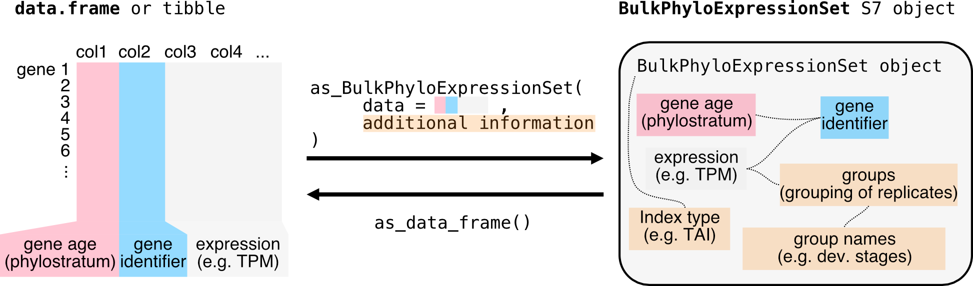
Now we construct the input data.frame for
as_BulkPhyloExpressionSet()
Show output
##            phylorank    GeneID    Zygote  Quadrant  Globular     Heart
## 1 Cellular Organisms AT1G01090 11424.567 16778.168 34366.649 39775.641
## 2 Cellular Organisms AT1G01620  5879.892  4977.186 11613.344  7295.212
## 3 Cellular Organisms AT1G01910  6644.138  6081.019  5130.440  5406.838
## 4 Cellular Organisms AT1G02305 14799.835 19609.824  6599.929  5535.103
## 5 Cellular Organisms AT1G02560  9915.822  9965.721 19602.787 22256.097
## 6 Cellular Organisms AT1G02730 15164.101 13536.758 12995.267 13102.109
##     Torpedo      Bent    Mature
## 1 56231.569 66980.367  7772.562
## 2 17289.631 11439.765  8183.609
## 3  5912.746  6820.958 10914.040
## 4  4785.300  3071.470  3916.300
## 5 27314.341 19444.084 13198.600
## 6 11251.254 14423.060 14051.317
## 'data.frame': 1757 obs. of 9 variables:
## $ phylorank: Factor w/ 19 levels "Cellular Organisms",..: 1 1 1 1 1 1 1 1 1 1 ...
## $ GeneID : chr "AT1G01090" "AT1G01620" "AT1G01910" "AT1G02305" ...
## $ Zygote : num 11425 5880 6644 14800 9916 ...
## $ Quadrant : num 16778 4977 6081 19610 9966 ...
## $ Globular : num 34367 11613 5130 6600 19603 ...
## $ Heart : num 39776 7295 5407 5535 22256 ...
## $ Torpedo : num 56232 17290 5913 4785 27314 ...
## $ Bent : num 66980 11440 6821 3071 19444 ...
## $ Mature : num 7773 8184 10914 3916 13199 ...Requirements for the input data.frame to the
as_BulkPhyloExpressionSet() function:
column 1 contains the phylorank information, which can be either numeric
or factors.
column 2 contains the gene identifier (here called
GeneID).
column 3 onwards contain the expression data with the column titles
being the developmental stages or the experimental conditions.
The example example_phyex_set.df is now formatted to
meet the requirements for the as_BulkPhyloExpressionSet()
function.
The BulkPhyloExpressionSet_from_df() function will
automatically detect the first column as the phylorank and the second
column as the gene identifier. If your data is structured differently,
you can reassign the columns accordingly using
dplyr::relocate().
Now, we can use the BulkPhyloExpressionSet_from_df()
function to convert the correctly formatted input
data.frame to a BulkPhyloExpressionSet
object.
There you have it, a BulkPhyloExpressionSet object!
example_phyex_set.remakeShow output
## PhyloExpressionSet object
## Class: myTAI::BulkPhyloExpressionSet
## Name: reconstituted phyex_set_old
## Species: NA
## Index type: TXI
## Identities : Zygote, Quadrant, Globular, Heart, Torpedo, Bent, Mature
## Number of genes: 1757
## Number of identities : 7
## Number of phylostrata: 19
## Number of samples: 7
## Samples per condition: 1 1 1 1 1 1 1
You can further explore the properties of the
BulkPhyloExpressionSet object using the @
operator, for example:
example_phyex_set.remake@counts |> head().
… and plot your transcriptome age index!
example_phyex_set.remake |>
    myTAI::plot_signature()
## Computing: [========================================] 100% (done)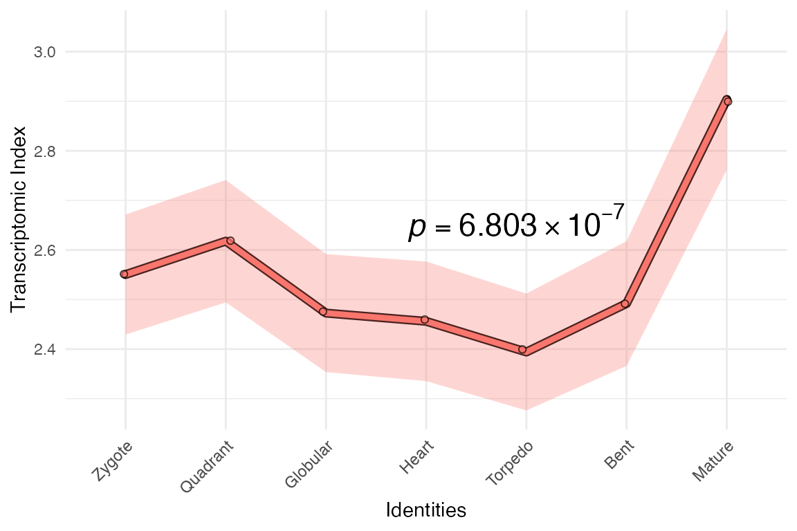
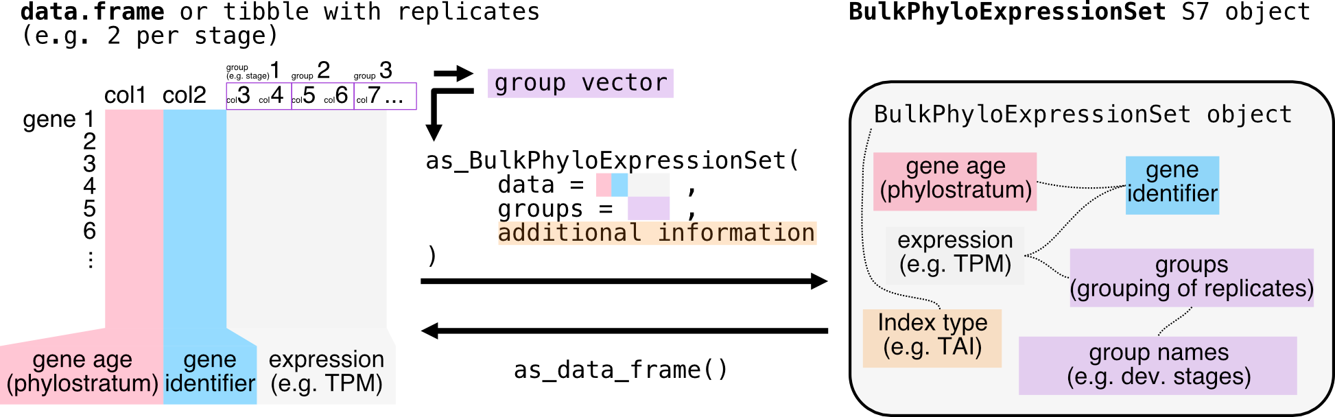
What if the dataset contains replicates?
This is exactly the case for the new example_phyex_set
dataset (not like example_phyex_set_old), which contains
replicates for each developmental stage. The
as_BulkPhyloExpressionSet() function can handle this as
well, as long as we use the groups parameter to specify the
grouping of replicates, i.e.
colnames(example_phyex_set.df)Show output
##  [1] "phylorank" "GeneID"    "pg_1"      "pg_2"      "pg_3"      "gl_1"
##  [7] "gl_2"      "gl_3"      "eh_1"      "eh_2"      "eh_3"      "lh_1"
## [13] "lh_2"      "lh_3"      "et_1"      "et_2"      "et_3"      "lt_1"
## [19] "lt_2"      "lt_3"      "bc_1"      "bc_2"      "bc_3"      "mg_1"
## [25] "mg_2"      "mg_3"
As you can see, this dataset has three replicates per stage.
Done!
Along with the groups parameter, you can also specify
the name, strata_labels and other parameters
to provide more descriptions for your
BulkPhyloExpressionSet object. This is useful for plotting
and visualisation purposes. Check this using ? before the
function (i.e. ?myTAI::as_BulkPhyloExpressionSet()).
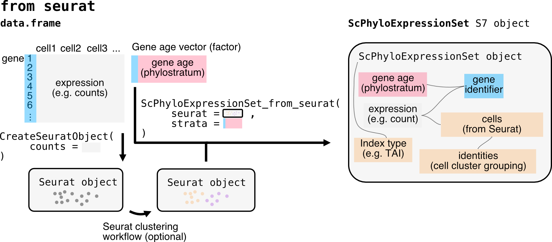
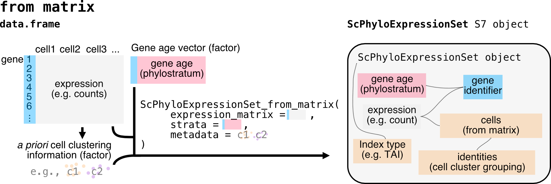
Mock single-cell dataset for ScPhyloExpressionSet
If you are interested in single cell RNA-seq data, the process is
similar, but you will need to ensure that your data is structured
correctly for single cell analysis, i.e. as a seurat object.
You can then use the ScPhyloExpressionSet_from_seurat()
or ScPhyloExpressionSet_from_matrix function with
adjustments to the relevant metadata.
# Load the relevant packages
library(dplyr)
library(Seurat)

pbmc_raw <- read.table(
  file = system.file('extdata', 'pbmc_raw.txt', package = 'Seurat'),
  as.is = TRUE
)
The input file for Seurat::CreateSeuratObject() is a
tab-separated file with the first column as gene identifiers and the
rest of the columns as expression values for each cell. The
pbmc_raw object is a data frame with gene expression
data.
head(pbmc_raw)Show output
## ATGCCAGAACGACT CATGGCCTGTGCAT GAACCTGATGAACC TGACTGGATTCTCA
## MS4A1 0 0 0 0
## CD79B 1 0 0 0
## CD79A 0 0 0 0
## HLA-DRA 0 1 0 0
## TCL1A 0 0 0 0
## HLA-DQB1 1 0 0 0
## AGTCAGACTGCACA TCTGATACACGTGT TGGTATCTAAACAG GCAGCTCTGTTTCT
## MS4A1 0 0 0 0
## CD79B 0 0 0 0
## CD79A 0 0 0 0
## HLA-DRA 1 1 0 1
## TCL1A 0 0 0 0
## HLA-DQB1 0 0 0 0
## GATATAACACGCAT AATGTTGACAGTCA AGGTCATGAGTGTC AGAGATGATCTCGC
## MS4A1 0 0 2 2
## CD79B 0 1 2 4
## CD79A 0 0 0 5
## HLA-DRA 0 0 14 28
## TCL1A 0 0 3 0
## HLA-DQB1 0 0 1 6
## GGGTAACTCTAGTG CATGAGACACGGGA TACGCCACTCCGAA CTAAACCTGTGCAT
## MS4A1 4 4 2 3
## CD79B 3 3 2 3
## CD79A 2 2 5 8
## HLA-DRA 18 7 15 28
## TCL1A 2 4 0 0
## HLA-DQB1 2 2 2 8
## GTAAGCACTCATTC TTGGTACTGAATCC CATCATACGGAGCA TACATCACGCTAAC
## MS4A1 3 4 2 3
## CD79B 1 2 2 5
## CD79A 1 5 5 12
## HLA-DRA 7 26 10 16
## TCL1A 3 3 3 2
## HLA-DQB1 2 2 1 2
## TTACCATGAATCGC ATAGGAGAAACAGA GCGCACGACTTTAC ACTCGCACGAAAGT
## MS4A1 0 0 0 0
## CD79B 0 0 0 0
## CD79A 0 0 1 0
## HLA-DRA 7 22 0 10
## TCL1A 0 0 0 0
## HLA-DQB1 0 3 0 0
## ATTACCTGCCTTAT CCCAACTGCAATCG AAATTCGAATCACG CCATCCGATTCGCC
## MS4A1 1 0 0 0
## CD79B 0 0 0 0
## CD79A 0 0 0 1
## HLA-DRA 6 0 4 3
## TCL1A 0 0 0 0
## HLA-DQB1 0 0 1 0
## TCCACTCTGAGCTT CATCAGGATGCACA CTAAACCTCTGACA GATAGAGAAGGGTG
## MS4A1 0 0 0 0
## CD79B 0 1 1 0
## CD79A 0 0 0 0
## HLA-DRA 7 13 0 1
## TCL1A 0 0 0 0
## HLA-DQB1 1 0 0 0
## CTAACGGAACCGAT AGATATACCCGTAA TACTCTGAATCGAC GCGCATCTTGCTCC
## MS4A1 0 0 0 0
## CD79B 2 0 0 0
## CD79A 0 0 0 0
## HLA-DRA 0 0 1 0
## TCL1A 0 0 0 0
## HLA-DQB1 0 0 0 0
## GTTGACGATATCGG ACAGGTACTGGTGT GGCATATGCTTATC CATTACACCAACTG
## MS4A1 0 0 0 0
## CD79B 0 0 0 0
## CD79A 0 0 0 0
## HLA-DRA 1 1 0 0
## TCL1A 0 0 0 0
## HLA-DQB1 0 0 0 0
## TAGGGACTGAACTC GCTCCATGAGAAGT TACAATGATGCTAG CTTCATGACCGAAT
## MS4A1 0 0 0 0
## CD79B 0 0 0 0
## CD79A 0 0 0 0
## HLA-DRA 0 0 0 0
## TCL1A 0 0 0 0
## HLA-DQB1 0 0 0 0
## CTGCCAACAGGAGC TTGCATTGAGCTAC AAGCAAGAGCTTAG CGGCACGAACTCAG
## MS4A1 0 0 0 0
## CD79B 0 0 0 0
## CD79A 0 0 0 0
## HLA-DRA 0 1 1 1
## TCL1A 0 0 0 0
## HLA-DQB1 0 0 0 0
## GGTGGAGATTACTC GGCCGATGTACTCT CGTAGCCTGTATGC TGAGCTGAATGCTG
## MS4A1 0 0 0 0
## CD79B 0 0 1 0
## CD79A 0 0 0 0
## HLA-DRA 0 0 10 10
## TCL1A 0 0 0 0
## HLA-DQB1 0 0 0 1
## CCTATAACGAGACG ATAAGTTGGTACGT AAGCGACTTTGACG ACCAGTGAATACCG
## MS4A1 0 0 0 0
## CD79B 1 1 2 2
## CD79A 0 0 0 0
## HLA-DRA 4 1 6 28
## TCL1A 0 0 0 0
## HLA-DQB1 1 0 2 0
## ATTGCACTTGCTTT CTAGGTGATGGTTG GCACTAGACCTTTA CATGCGCTAGTCAC
## MS4A1 0 0 0 0
## CD79B 0 0 3 0
## CD79A 0 0 0 0
## HLA-DRA 10 13 5 8
## TCL1A 0 0 0 0
## HLA-DQB1 0 1 1 0
## TTGAGGACTACGCA ATACCACTCTAAGC CATATAGACTAAGC TTTAGCTGTACTCT
## MS4A1 0 0 0 0
## CD79B 0 0 0 4
## CD79A 0 0 0 8
## HLA-DRA 108 93 41 42
## TCL1A 0 0 0 4
## HLA-DQB1 21 21 3 5
## GACATTCTCCACCT ACGTGATGCCATGA ATTGTAGATTCCCG GATAGAGATCACGA
## MS4A1 0 0 0 1
## CD79B 1 0 0 0
## CD79A 0 0 0 0
## HLA-DRA 138 77 76 15
## TCL1A 0 0 0 0
## HLA-DQB1 11 11 10 1
## AATGCGTGGACGGA GCGTAAACACGGTT ATTCAGCTCATTGG GGCATATGGGGAGT
## MS4A1 0 0 0 0
## CD79B 0 0 0 0
## CD79A 1 0 0 0
## HLA-DRA 19 104 1 0
## TCL1A 0 0 0 0
## HLA-DQB1 2 11 0 0
## ATCATCTGACACCA GTCATACTTCGCCT TTACGTACGTTCAG GAGTTGTGGTAGCT
## MS4A1 0 0 0 0
## CD79B 0 0 0 0
## CD79A 0 0 0 0
## HLA-DRA 0 0 2 1
## TCL1A 0 0 0 0
## HLA-DQB1 0 0 0 0
## GACGCTCTCTCTCG AGTCTTACTTCGGA GGAACACTTCAGAC CTTGATTGATCTTC
## MS4A1 0 0 0 0
## CD79B 0 0 0 0
## CD79A 0 0 0 0
## HLA-DRA 1 0 2 7
## TCL1A 0 0 0 0
## HLA-DQB1 0 0 0 1Now, we create a Seurat object. i.e.
pbmc_small <- CreateSeuratObject(counts = pbmc_raw)
is(pbmc_small)## [1] "Seurat"Now, we can convert this Seurat object to a
ScPhyloExpressionSet object using the
ScPhyloExpressionSet_from_seurat() function.
The next part is a bit tricky, as you need to provide the phylorank
information in a specific format with the same gene identifiers as that
of pbmc_small.
We will generate random phyloranks for each gene as integers.
gene_names <- pbmc_small |> rownames()
example_phylorank_sc <-
    setNames(sample(1:10, length(gene_names), replace = TRUE), gene_names) |>
    as.factor()
example_phyex_set_sc <-
    myTAI::ScPhyloExpressionSet_from_seurat(
        pbmc_small,
        strata = example_phylorank_sc)
Example of a downstream analysis
Here, we will go a bit deeper and cluster the pbmc_small
object before integrating this to the myTAIv2 workflow.
# example workflow to cluster the single cell data
pbmc_small <- Seurat::NormalizeData(pbmc_small)
pbmc_small <- Seurat::FindVariableFeatures(pbmc_small, selection.method = "vst", nfeatures = 20)
pbmc_small <- Seurat::ScaleData(pbmc_small)
pbmc_small <- Seurat::RunPCA(pbmc_small, features = VariableFeatures(object = pbmc_small))
pbmc_small <- Seurat::FindNeighbors(pbmc_small, dims = 1:10)
pbmc_small.cluster <- Seurat::FindClusters(pbmc_small, resolution = 0.8)
## Modularity Optimizer version 1.3.0 by Ludo Waltman and Nees Jan van Eck
##
## Number of nodes: 80
## Number of edges: 2352
##
## Running Louvain algorithm...
## Maximum modularity in 10 random starts: 0.4014
## Number of communities: 2
## Elapsed time: 0 seconds
example_phyex_set_sc.cluster <-
    myTAI::ScPhyloExpressionSet_from_seurat(
        seurat = pbmc_small.cluster,
        strata = example_phylorank_sc)
Now we have the ScPhyloExpressionSet object,
example_phyex_set_sc.cluster… which you can now plot!
myTAI::plot_signature(example_phyex_set_sc.cluster)## Warning: Using `size` aesthetic for lines was deprecated in ggplot2 3.4.0.
## ℹ Please use `linewidth` instead.
## ℹ The deprecated feature was likely used in the myTAI package.
## Please report the issue at <https://github.com/drostlab/myTAI/issues>.
## This warning is displayed once per session.
## Call `lifecycle::last_lifecycle_warnings()` to see where this warning was
## generated.## Computing: [========================================] 100% (done)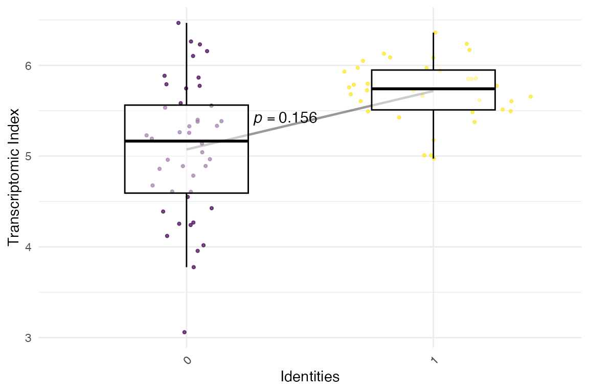
This example used an example Seurat object with a mock phylorank dataset (random gene age assignment) and an example workflow. In practice, you will have to follow the best standards for single cell RNA-seq data analysis, including quality control, normalisation, and clustering steps. And assign real phylorank information to the genes in your dataset (to do this, see the phylostratigraphy vignette).
Summary
In this section, we have learned how to create
BulkPhyloExpressionSet and
ScPhyloExpressionSet objects from raw gene expression data
and phylorank information. This object is essential for performing
evolutionary transcriptomics analyses using the myTAI
package, and provides a structured way to store and manipulate
evolutionary transcriptomics data, making it easier to perform various
analyses and visualisations.